

This post presents the procedure in scaling of base shear in ETABS. It is assumed that you are already aware of the principles of response spectrum analysis and are using CSI ETABS as your analysis tool.
UBC-97 and ASCE 7-05 or later require that the base shear calculated using modal response spectrum dynamic analysis should exceed or match a certain percentage of the static base shear calculated using Equivalent Lateral Force procedure (static analysis). The requirements of ASCE 7-05 are implemented in this example. For completeness, relevant steps on how to set up the spectrum cases in ETABS are presented.
STEP 1:
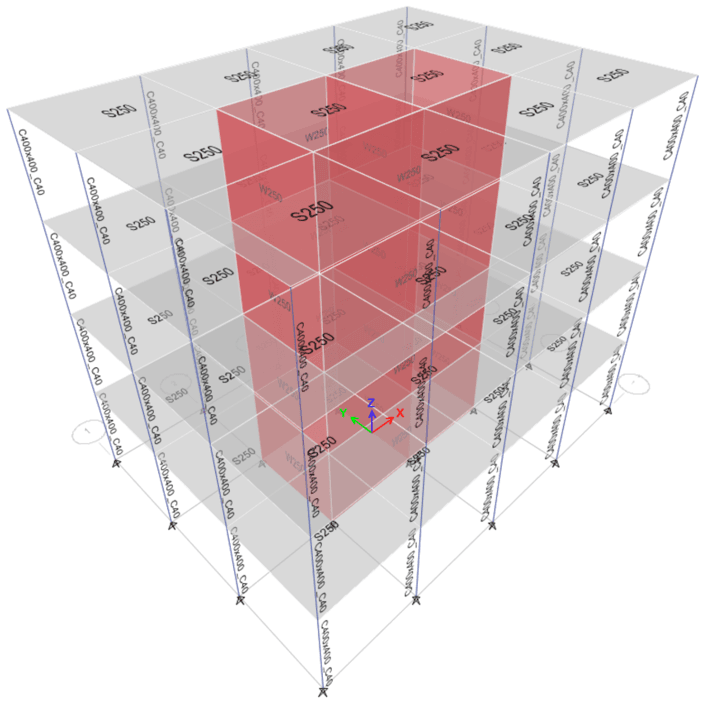
An ETABS model should already be available for the project.

STEP 2:
Declare the static load cases in x- and y-direction. In this example, these are designated as EQX and EQY respectively.
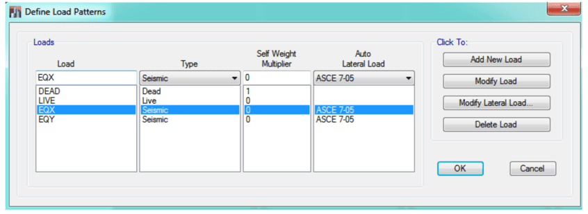
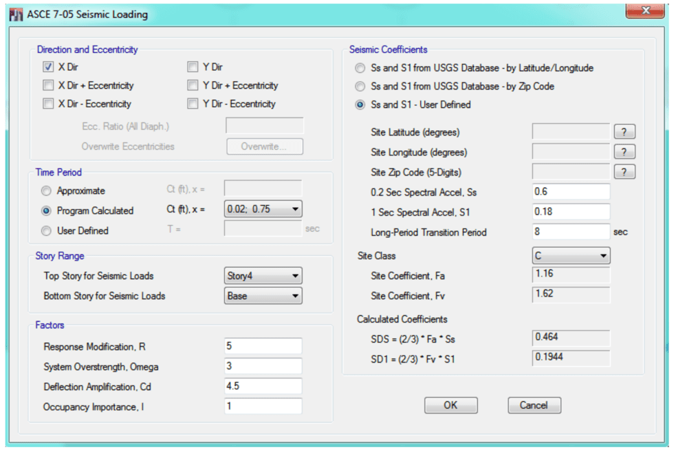
The seismic parameters are project specific dependent on seismicity of the region, the underlying soil class and type of building structure. Eccentricity in seismic loading will not be considered for the static cases since the base shear obtained from EQX and EQY cases would only be used for base shear scaling and not for design, i.e. seismic design will only use the forces from dynamic analysis.
STEP 3:
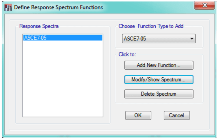
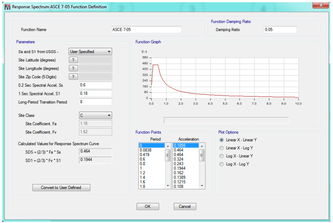
Define the Response Spectrum function. The parameters you input here should match the static case seismic parameters.
STEP 4:
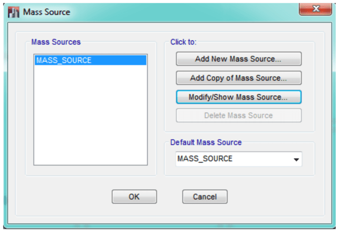
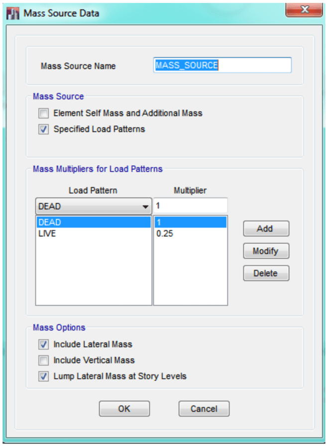
Define the mass source to be used in the seismic analysis specific to the project criteria. For example, you might include 25% of the occupancy live load as part of the mass source.
STEP 5:
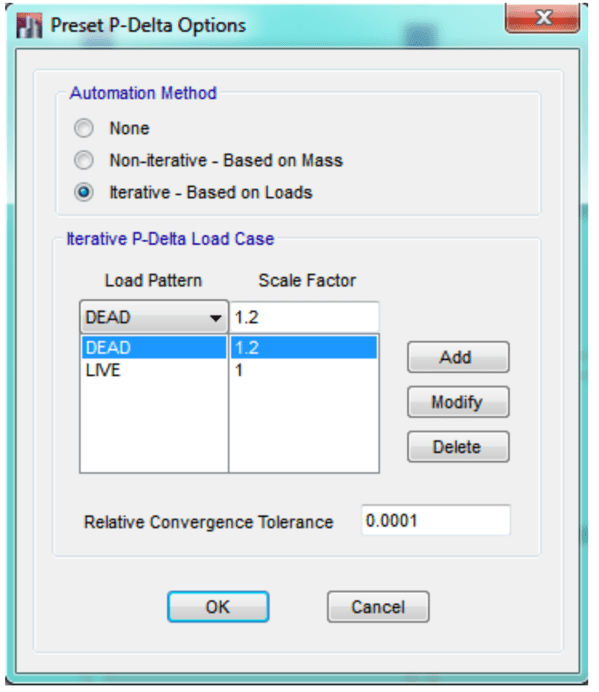
Define the P-delta parameters based on project specific criteria or standard practice. Usually, the factors of the gravity load component of the governing seismic load combination is used. For example, if the load combination includes 1.2 DEAD + 1.0 LIVE + 1.0 EARTHQUAKE, and deem that the gravity component of this combination would produce the highest P-delta effect, you would input:
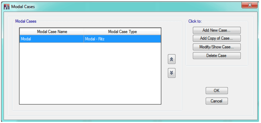
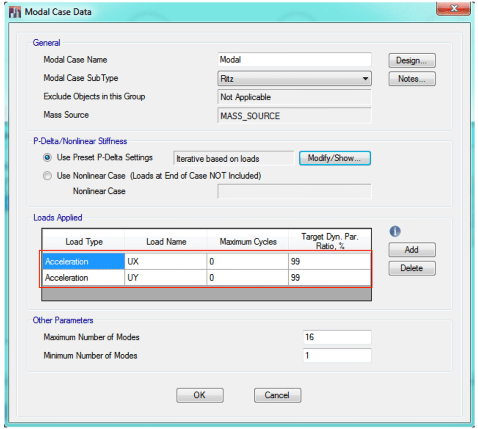
STEP 6:
Set up the modal case which must include vibration in both x- and y-direction. There should be sufficient number of modes to achieve at such that at least 90% total mass participation (ASCE 7-05 Section 12.9.1). In this example, Ritz method is used with 16 modes analyzed.
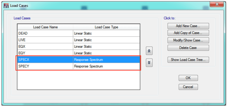
STEP 7:
Add two Response Spectrum cases in U1 and U2 horizontal direction. In this example, SPECX and SPECY are defined respectively.
The response spectra is to be multiplied g/R*I (ASCE 7-05 Section 12.9.2), hence an initial scale should be entered for each response spectrum case. Note that by defining an initial scale as a factor of g, the results obtained from the response spectrum analysis would be a force value, e.g. in kN unit.
Sample calculation of initial scale computation:
Scale,initial = 9806.65 mm/s^2 / 5.0 * 1.0 = 1961
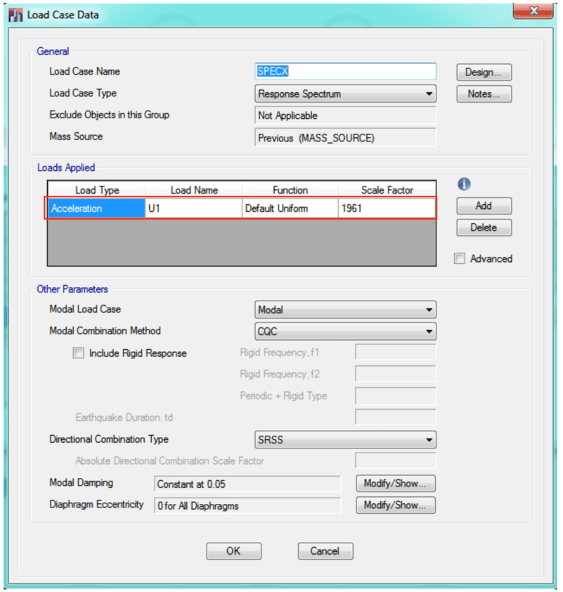
The adopted method for modal combination is CQC while the directional combination is SRSS.
STEP 8:
Create a load combination that combines the response from each direction SPECX and SPECY. Two methods are commonly used:
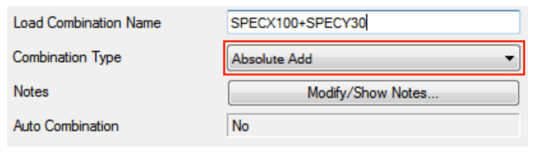
- Method 1) 100% from one direction + 30% from the other direction
- Method 2) Square root of the sum of squares (SRSS) of the effect from each direction.
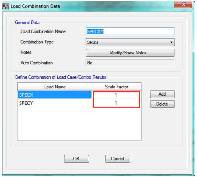
The SRSS method of combination will be used in this example. This is declared as SPECXY in the ETABS load combination definition.
For complex or irregular structures which do not have clearly defined orthogonal directions, it may be unclear as to how the orientation of response-spectrum analysis should be applied. In the paper entitled Orthogonal Effects in RSA , Dr. Wilson explains that combined directional effects may be accounted for more effectively by using an alternative method in which the SRSS combination of two 100-percent spectra analyses is applied in any direction, or along either orthogonal axis.
CSI Knowledge Base
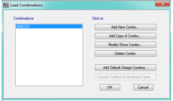
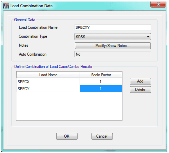
Scale values of 1.0 are applied for each case. This can be adjusted later in the load combination of SPECXY after the analysis has been completed. If a higher scale factor is necessary to satisfy code requirements, this can be applied in the combination without having to rerun the dynamic analysis. This can save hours or even days of computer analysis time in case of a huge model!
NOTE: If Method 1 combination is preferred, the “Absolute Add” combination type should be selected:
STEP 9:
If you have completed STEPS 1-8, you should be able to run the analysis. After the analysis is completed, click on Display > Show Tables
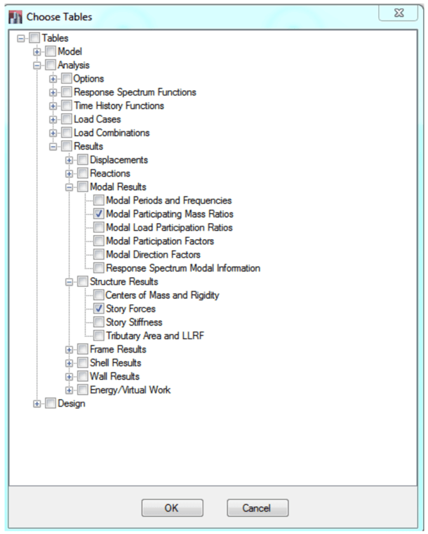
and Analysis > Results > Structure Results > Story Forces check boxes.
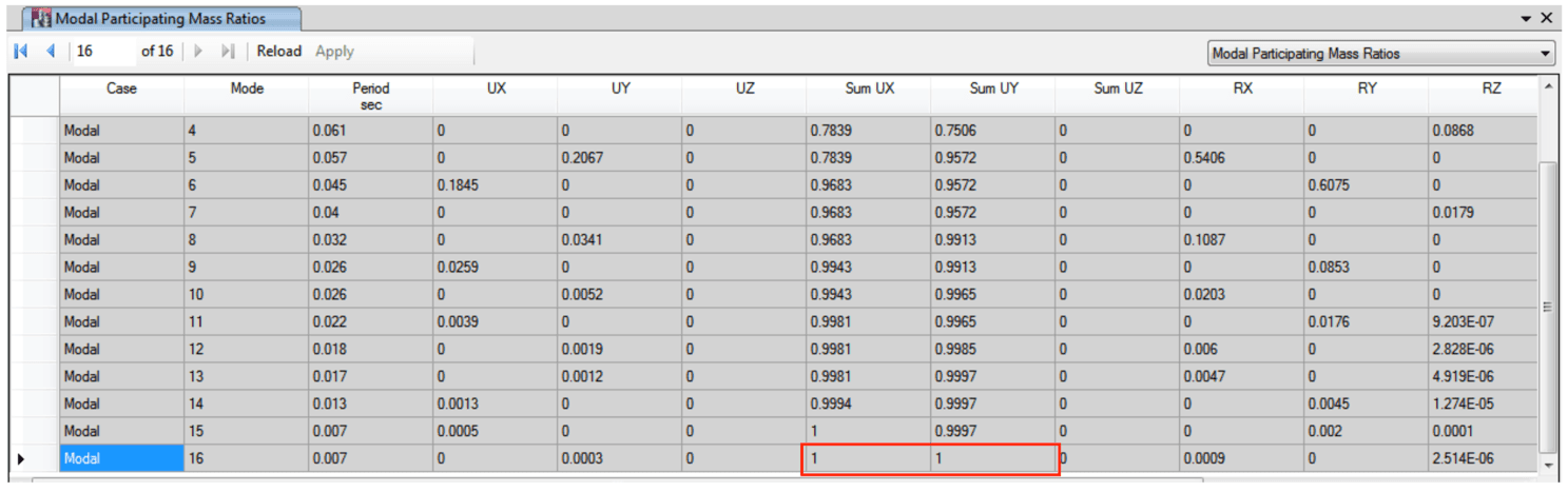
Select the “Modal Participating Mass Ratios” table. Verify that both “Sum UX” and “Sum UY” have achieved at least 90% participation. If not, increase the number of modes then rerun the analysis. For our example, 100% participation has been achieved.
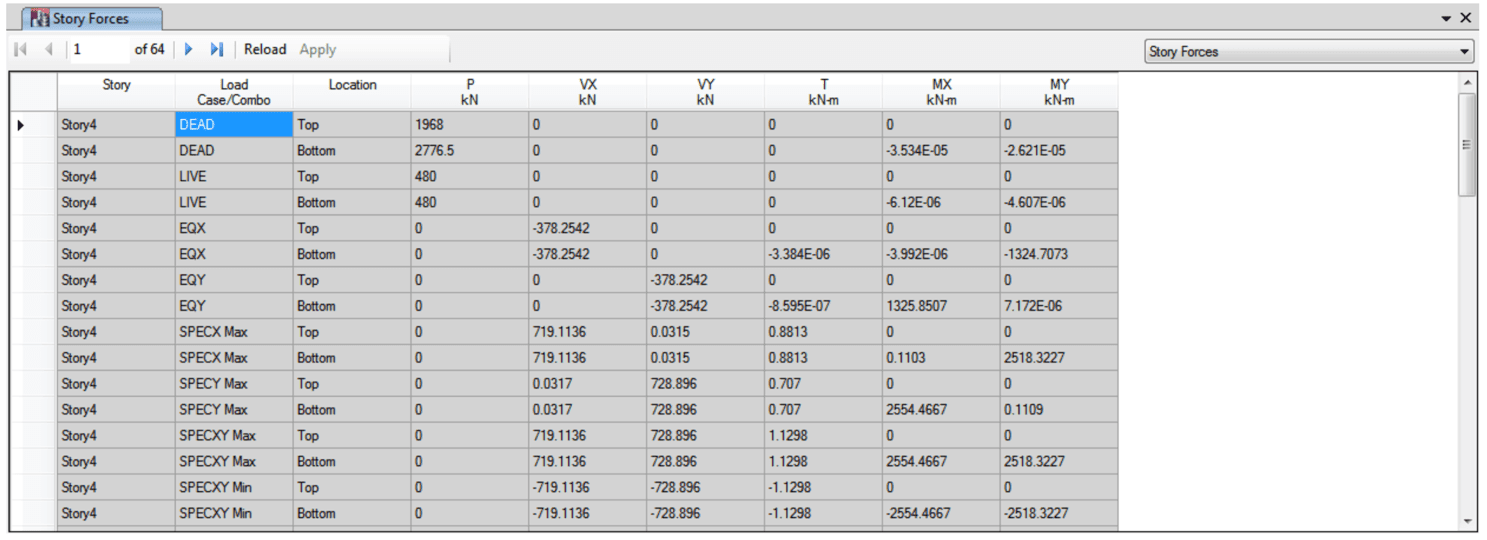
Select the “Story Forces” table. Right-click on any part of the table and choose “Export to Excel”
STEP 10:
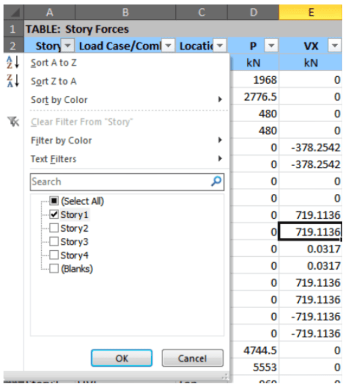
With the data exported in Excel, filter the data by clicking Data > Filter

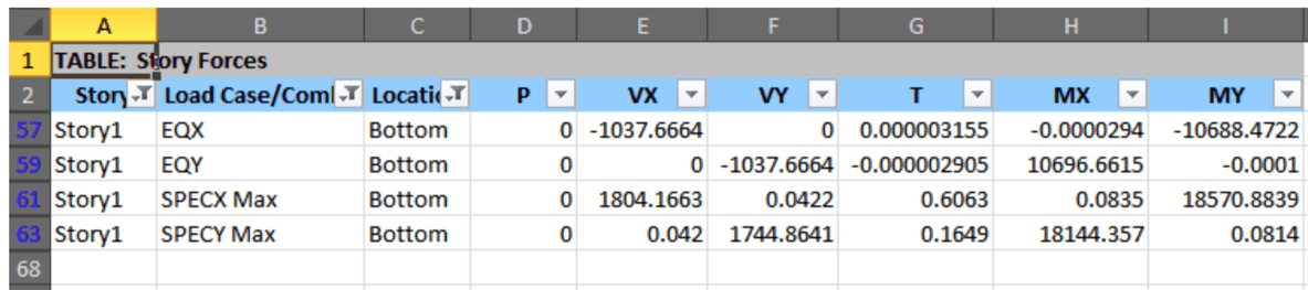
The base shear will be scaled from the base of the structure, therefore select the lowest level only. In our example, Story1.
Filter the Load Case/Combo by selecting EQX, EQY, SPECX Max, and SPECY Max.
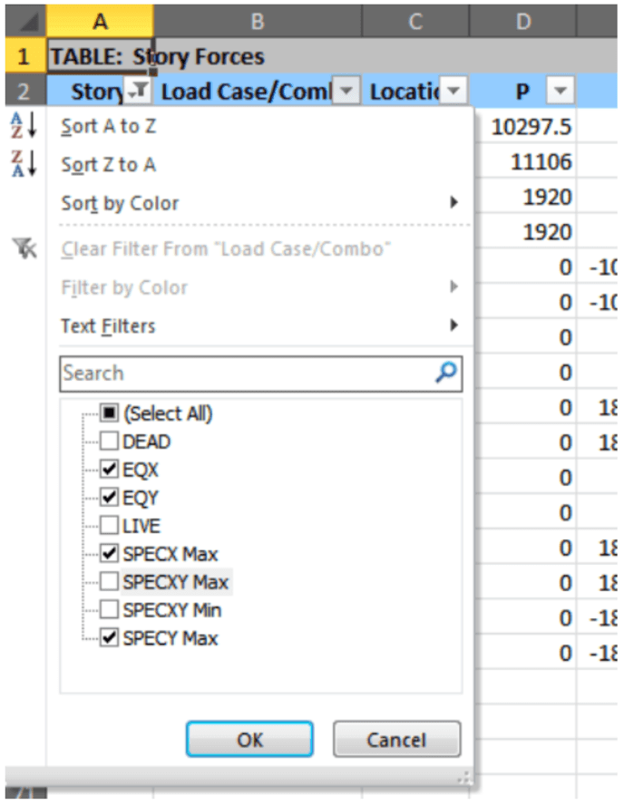
Finally, filter Location to display the Bottom forces only. The Excel table should now look like as shown:
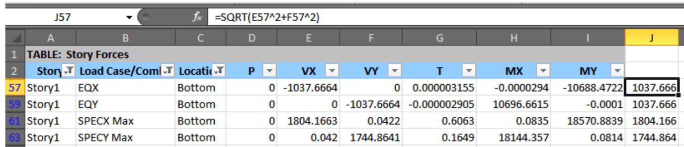
Create a formula at the end of each row to calculate the resultant shear:
SQRT(VX^2 + VY^2)
Get the ratio between dynamic and static base shear. In this example,
Ratio,x = VSPECX/VEQX = 1804.166/1037.666
Ratio,x = 1.739
Ratio,y = VSPECY/VEQY = 1744.864/1037.666
Ratio,y = 1.682
The ratio should be greater than the minimum prescribed by the code. Based on ASCE 7-05 Section 12.9.4, the ratio should be more than 85%. Since both Ratio,x and Ratio,y are greater than 0.85, there is no need to further adjust the scales, e.g. keep SPECX=1 and SPECY=1 under the load combination SPECXY.
Create other seismic load combinations in ETABS and make use of the pre-combined SPECXY load combination. For example, the ASCE 7-05 combination
1.2 DEAD + 1.0 EQ + 1.0 LIVE
can be defined in ETABS as shown:
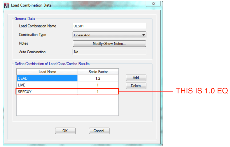
Notice how we used the combined effect SPECXY instead of SPECX or SPECY individually. This reduces the total number of seismic combinations we would need to define in ETABS. ASCE 7-05 also requires us to include the vertical component of the earthquake force in the combination (not shown in this simple example).
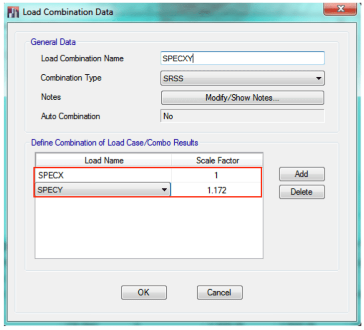
STEP11:
What if the ratio between dynamic and static base shear is less than 0.85? Let’s consider the following data derived from another theoretical ETABS analysis.
V,EQX = 10800 kN
V,EQY = 10800 kN
V,SPECX = 9850 kN
V,SPECY = 7830 kN

Ratio,x = 9850/10800 = 0.912 > 0.85, ok (don't reduce scale!)
Ratio,y = 7830/10800 = 0.725 < 0.85, scale up!

Scale,SPECX = 1.0
Scale,SPECY = 0.85/0.725 = 1.172
This means that we need to scale up the factors as follows :
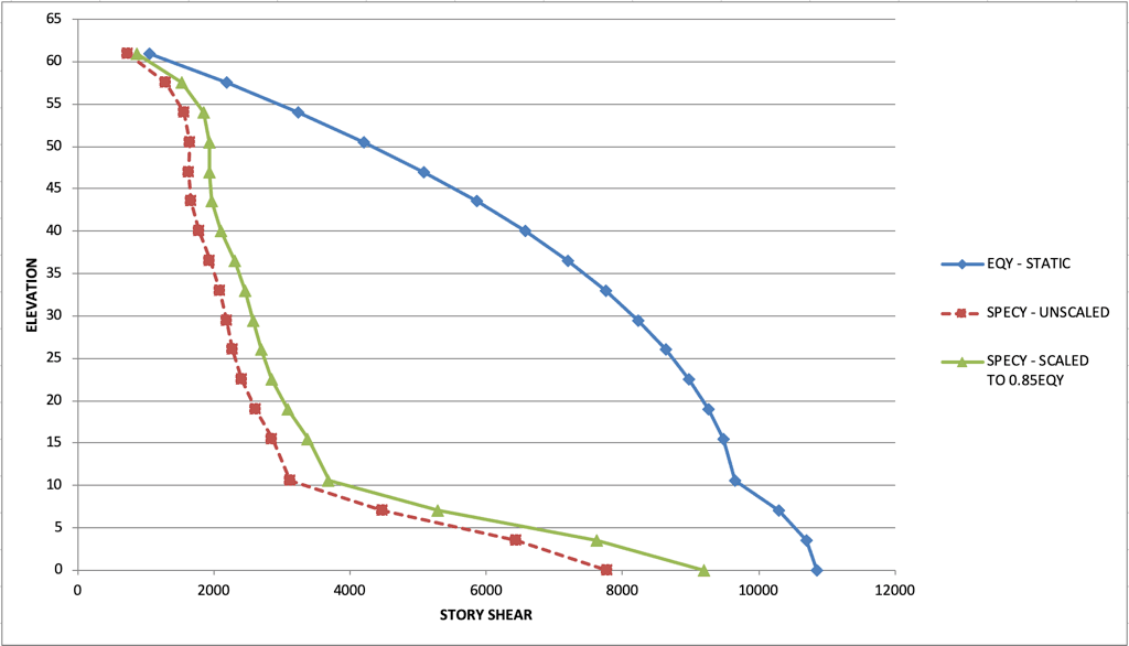
The above diagram shows the original unscaled dynamic story shear (red lines) and the scaled up dynamic story shear (green lines). In this example, it can be seen that the shear force distribution for each corresponding story is lower in the dynamic analysis procedure as compared with the static analysis procedure. This is generally the case, therefore most structural designers prefer to apply dynamic seismic analysis which could result to more economical design.